

How to Build a Python Tool for Diagnosing Diseases with Medical Imaging and Deep Learning
Learn how to develop a Python tool that uses deep learning and medical imaging to diagnose diseases through X-rays, MRIs, and CT scans
Medical imaging has been revolutionized by deep learning, enabling automated diagnosis from scans such as X-rays, CT scans, or MRIs. This guide will walk through the steps of creating a Python tool to diagnose diseases using medical images and deep learning models, including the necessary libraries, dataset usage, and model training process.
1. Setting Up the Environment
Before diving into coding, you need to install some key libraries to handle image processing, deep learning, and data visualization.
pip install tensorflow keras opencv-python matplotlib numpy
TensorFlow/Keras: The deep learning framework used for building and training the neural network.
OpenCV: For image manipulation and preprocessing.
Matplotlib: For visualizing data and model performance.
NumPy: For efficient numerical computation.
2. Dataset Collection and Preprocessing
a. Downloading a Dataset:
You can find medical imaging datasets on platforms like Kaggle. For this example, let's assume we're working with a Chest X-ray dataset to detect pneumonia.
kaggle datasets download -d paultimothymooney/chest-xray-pneumonia
After downloading the dataset, extract the files and organize them into training and testing directories.
b. Image Preprocessing:
Preprocessing is crucial to ensure that the images are in the right format for model training. Here’s how to load and preprocess images:
import os
import cv2
import numpy as np
import matplotlib.pyplot as plt

# Directory containing the dataset
train_dir = 'chest_xray/train/'
test_dir = 'chest_xray/test/'

# Image size expected by the model
IMG_SIZE = 150

def preprocess_image(img_path):
    # Load the image in grayscale
    img = cv2.imread(img_path, cv2.IMREAD_GRAYSCALE)
    # Resize to the required dimensions
    img = cv2.resize(img, (IMG_SIZE, IMG_SIZE))
    # Normalize the image
    img = img / 255.0
    return img

# Example of loading and displaying an image
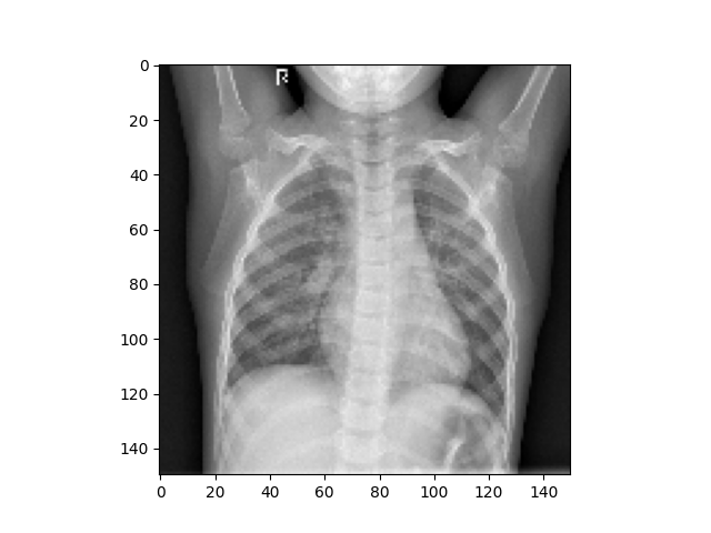
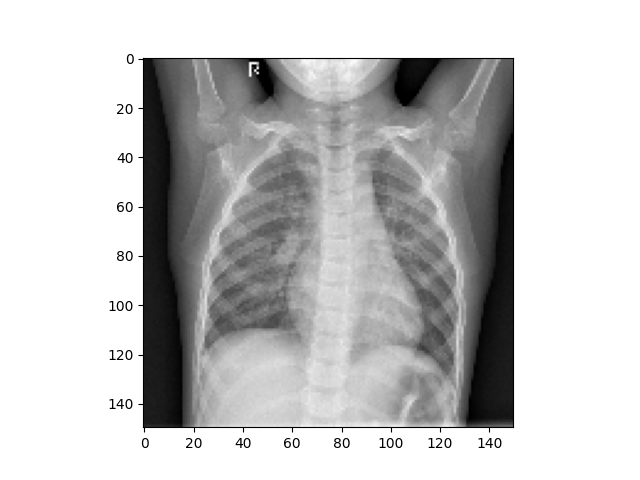
sample_image = preprocess_image(train_dir + 'NORMAL/IM-0115-0001.jpeg')
plt.imshow(sample_image, cmap='gray')
plt.show()
3. Building the Deep Learning Model
Now, we’ll build a convolutional neural network (CNN) to handle the medical images.
from tensorflow.keras.models import Sequential
from tensorflow.keras.layers import Conv2D, MaxPooling2D, Flatten, Dense, Dropout

# Define the CNN model
model = Sequential()

# First convolutional layer
model.add(Conv2D(32, (3, 3), activation='relu', input_shape=(IMG_SIZE, IMG_SIZE, 1)))
model.add(MaxPooling2D(pool_size=(2, 2)))

# Second convolutional layer
model.add(Conv2D(64, (3, 3), activation='relu'))
model.add(MaxPooling2D(pool_size=(2, 2)))

# Flatten the output of the convolutions
model.add(Flatten())

# Fully connected layer
model.add(Dense(128, activation='relu'))
model.add(Dropout(0.5))

# Output layer (Binary classification: Pneumonia or Not)
model.add(Dense(1, activation='sigmoid'))

# Compile the model
model.compile(optimizer='adam', loss='binary_crossentropy', metrics=['accuracy'])
4. Data Augmentation and Training
To avoid overfitting and improve the model's generalization, we use data augmentation techniques like rotation and zoom.
from tensorflow.keras.preprocessing.image import ImageDataGenerator

# Create an ImageDataGenerator for augmentation
datagen = ImageDataGenerator(
    rotation_range=15,
    zoom_range=0.2,
    horizontal_flip=True,
    validation_split=0.2  # Use a portion of training data for validation
)

# Load the images from the directories and apply augmentation
train_generator = datagen.flow_from_directory(
    train_dir,
    target_size=(IMG_SIZE, IMG_SIZE),
    color_mode='grayscale',
    batch_size=32,
    class_mode='binary',
    subset='training'  # Training data
)

validation_generator = datagen.flow_from_directory(
    train_dir,
    target_size=(IMG_SIZE, IMG_SIZE),
    color_mode='grayscale',
    batch_size=32,
    class_mode='binary',
    subset='validation'  # Validation data
)

# Train the model
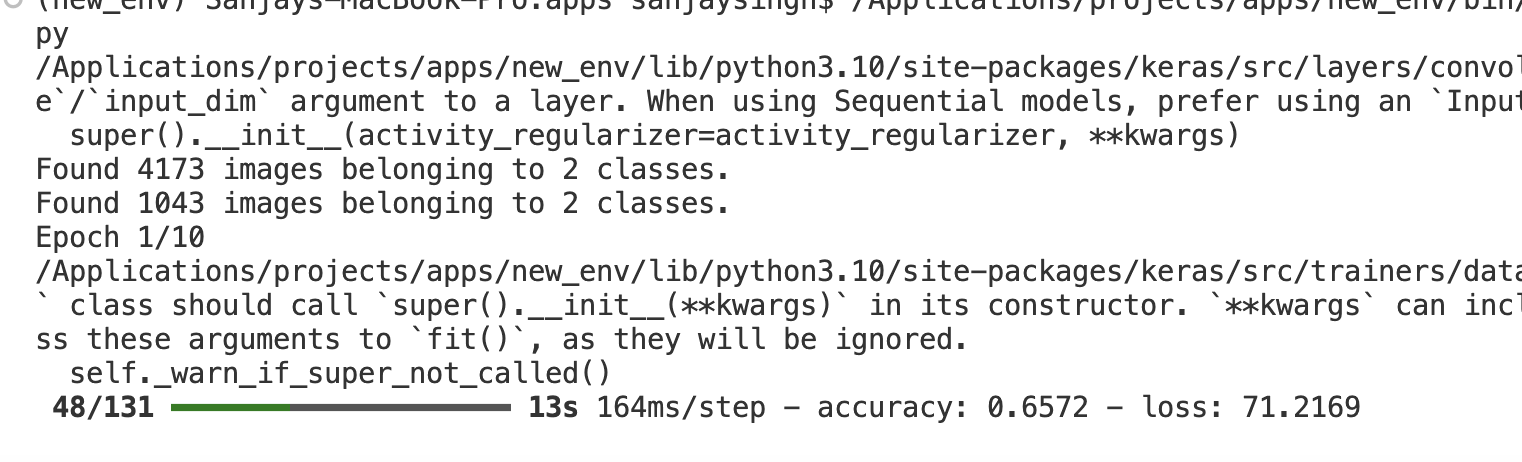
history = model.fit(
    train_generator,
    validation_data=validation_generator,
    epochs=10
)
5. Evaluating the Model
Once the model is trained, it’s essential to evaluate it on the test set to see how it performs on unseen data.
test_datagen = ImageDataGenerator()

test_generator = test_datagen.flow_from_directory(
    test_dir,
    target_size=(IMG_SIZE, IMG_SIZE),
    color_mode='grayscale',
    batch_size=32,
    class_mode='binary'
)

# Evaluate the model on the test set
test_loss, test_accuracy = model.evaluate(test_generator)
print(f"Test Accuracy: {test_accuracy * 100:.2f}%")
6. Visualizing Model Performance
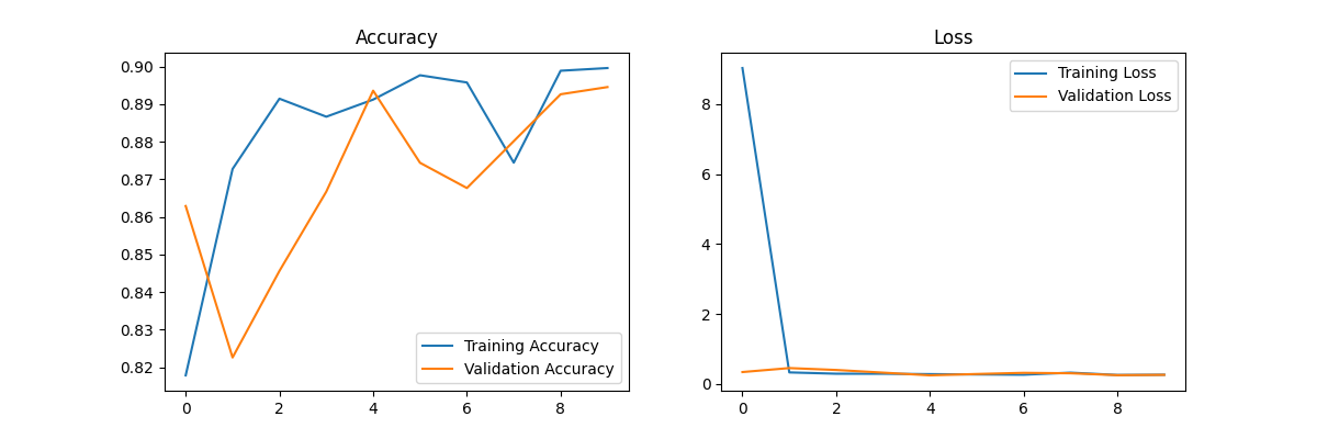
You can visualize the model's performance using the history object that Keras provides.
# Plot accuracy and loss curves
plt.figure(figsize=(12, 4))

# Accuracy plot
plt.subplot(1, 2, 1)
plt.plot(history.history['accuracy'], label='Training Accuracy')
plt.plot(history.history['val_accuracy'], label='Validation Accuracy')
plt.title('Accuracy')
plt.legend()

# Loss plot
plt.subplot(1, 2, 2)
plt.plot(history.history['loss'], label='Training Loss')
plt.plot(history.history['val_loss'], label='Validation Loss')
plt.title('Loss')
plt.legend()

plt.show()
7. Making Predictions
Once your model is trained and evaluated, you can use it to make predictions on new medical images.
# Load and preprocess a new image
new_image = preprocess_image('path_to_new_image.jpg')

# Add batch dimension and predict
new_image = np.expand_dims(new_image, axis=0)
prediction = model.predict(new_image)

# Interpret the result
if prediction[0][0] > 0.5:
    print("Pneumonia detected")
else:
    print("No Pneumonia detected")

Conclusion
About the author
Our company comprises seasoned professionals, each an expert in their field. Customer satisfaction is our top priority, exceeding clients' needs. We ensure competitive pricing and quality in web and mobile development without compromise.
Comments
Join the discussionpython in medical has a great scope in my opinion
Machine Learning
"Join us on a journey into the world of machine learning, where we unravel the complexities of algorithms, data processing, and model building."


